Tavex uses cookies to ensure website functionality and improve your user experience. Collecting data from cookies helps us provide the best experience for you, keeps your account secure and allows us to personalise advert content. You can find out more in our cookie policy.
Please select what cookies you allow us to use
Cookies are small files of letters and digits downloaded and saved on your computer or another device (for instance, a mobile phone, a tablet) and saved in your browser while you visit a website. They can be used to track the pages you visit on the website, save the information you enter or remember your preferences such as language settings as long as you’re browsing the website.
Cookie usage
Necessary cookies
| Cookie name | Cookie description | Cookie duration |
|---|---|---|
| tavex_cookie_consent | Stores cookie consent options selected | 60 weeks |
| tavex_customer | Tavex customer ID | 30 days |
| wp-wpml_current_language | Stores selected language | 1 day |
| AWSALB | AWS ALB sticky session cookie | 6 days |
| AWSALBCORS | AWS ALB sticky session cookie | 6 days |
| NO_CACHE | Used to disable page caching | 1 day |
| PHPSESSID | Identifier for PHP session | Session |
| latest_news | Helps to keep notifications relevant by storing the latest news shown | 29 days |
| latest_news_flash | Helps to keep notifications relevant by storing the latest news shown | 29 days |
| tavex_recently_viewed_products | List of recently viewed products | 1 day |
| tavex_compare_amount | Number of items in product comparison view | 1 day |
Preference cookies
| Cookie name | Cookie description | Cookie duration |
|---|---|---|
| chart-widget-tab-*-*-* | Remembers last chart options (i.e currency, time period, etc) | 29 days |
| archive_layout | Stores selected product layout on category pages | 1 day |
Targeting cookies
| Cookie name | Cookie description | Cookie duration |
|---|---|---|
| cartstack.com-* | Used for tracking abandoned shopping carts | 1 year |
| _omappvp | Used by OptinMonster for determining new vs. returning visitors. Expires in 11 years | 11 years |
| _omappvs | Used by OptinMonster for determining when a new visitor becomes a returning visitor | Session |
| om* | Used by OptinMonster to track interactions with campaigns | Persistent |
Analytical cookies
| Cookie name | Cookie description | Cookie duration |
|---|---|---|
| _ga | Used to distinguish users | 2 years |
| _gid | Used to distinguish users | 24 hours |
| _ga_* | Used to persist session state | 2 years |
| _gac_* | Contains campaign related information | 90 days |
| _gat_gtag_* | Used to throttle request rate | 1 minute |
| _fbc | Facebook advertisement cookie | 2 years |
| _fbp | Facebook cookie for distinguishing unique users | 2 years |

The Law of Supply and Demand
Published by Tavex Analysts in category Precious Metal Information Guides on 09.02.2024
Gold price (XAU-GBP)
3,032.15 GBP/oz
- GBP55.55
Silver price (XAG-GBP)
43.21 GBP/oz
- GBP2.00

The principle of supply and demand actually encompasses two distinct laws, which serve as the starting point for nearly every economics textbook. However, some educational series stands out by prioritising other crucial mechanisms before delving into these laws.
At its core, the principle of supply and demand forms the bedrock for our comprehension of the world around us, underpinning a multitude of phenomena observed in the marketplace.
We understand that value is inherently subjective, and it is the interplay of supply and demand that establishes market prices. In this discussion, we aim to delve into the origins of the law of supply and demand, examine its mechanics, and clarify what these terms signify within the realm of economics.
The Law of Demand
Looking at the concept presented by the law of supply and demand , we should start with demand. And with the law of demand.
Demand is the relationship between the consumption of a product or service and its varying prices
Simply put, demand illustrates the amount of a particular product consumers are prepared to purchase at differing price points. This concept applies to both individual consumers and groups.
The law of demand posits that, all else being equal, as the price of a product increases, the quantity consumed decreases. This inverse relationship is graphically represented by the demand curve, which slopes downward on a graph.
The demand curve visually maps out the quantity of a product that will be bought at various price levels, typically captured at a specific moment in time. On this graph, the quantity demanded is plotted on the horizontal axis (abscissa), while the price is charted on the vertical axis (ordinate).
How is the demand curve derived?
Let’s envision a scenario where various individuals are considering whether to purchase gold. Depending on the market price of gold at that moment, their respective demands would be as follows:
Table 1 : Demanded Quantity of Troy Ounces at the Relevant Price
| Price Per Troy Ounce ($) | Jen | Beth | Jim | David | Hank | Julian | Total Market Demand |
| 2500 | 0 | 0 | 0.5 | 1 | 13 | 0 | 14.5 |
| 2400 | 0 | 0 | 0.5 | 1.5 | 13 | 0 | 15 |
| 2300 | 0 | 0 | 1 | 2 | 13 | 0 | 16 |
| 2200 | 0 | 0 | 1 | 2.5 | 13 | 0 | 16.5 |
| 2100 | 0 | 0 | 1 | 3 | 13 | 0 | 17 |
| 1800 | 1.5 | 0 | 2 | 3 | 13 | 0 | 19.5 |
| 1700 | 2.5 | 0 | 2 | 5 | 13 | 0 | 22.5 |
| 1600 | 4 | 0 | 2 | 5 | 13 | 0 | 24.5 |
| 1500 | 8 | 0 | 4 | 5 | 13 | 0 | 30 |
| 1400 | 10.7 | 6.3 | 8 | 15 | 13 | 0 | 49 |
| 1300 | 14.7 | 6.3 | 8 | 15 | 13 | 0 | 57 |
| 1200 | 14.7 | 6.3 | 8 | 15 | 13 | 0 | 57 |
| 0 | 14.7 | 6.3 | 8 | 15 | 13 | 0 | 57 |
From this basis, we can also construct the demand curve for this market. Typically, demand curves are denoted with the Latin letter “D” for “demand”. As we will observe in the following illustrations, these curves are often stylised in graphical representations. This convention applies to the supply curve as well.
Graph 1 : Total Market Demand Curve
The Law of Supply
Continuing our examination of the law of supply and demand, we turn our attention to supply.
The law of supply is essentially the counterpart to the law of demand. It describes the relationship between the quantity of goods or services produced and their price in the market.
In essence, it specifies the amount of goods producers are prepared to supply at varying price levels. Holding all else constant, as the price escalates, so does the supply. This causal relationship is visually represented by the supply curve, denoted as “S” for “supply,” which is characterized by its upward slope.
Building on the previous scenario, let’s consider a market with three gold producers. At a certain price level for gold, they produce the following quantities:
Table 2 : Demanded Supply of Troy Ounces at the Relevant Price
| Price Per Troy Ounce ($) | GoldBest | GoldMax | GoldUltra | Total Market Supply (in Troy Ounces) |
| 2500 | 70 | 200 | 20 | 290 |
| 2400 | 55 | 200 | 20 | 275 |
| 2300 | 40 | 200 | 20 | 260 |
| 2200 | 30 | 180 | 0 | 210 |
| 2100 | 25 | 150 | 0 | 175 |
| 1800 | 19 | 120 | 0 | 139 |
| 1700 | 17 | 100 | 0 | 117 |
| 1600 | 15 | 50 | 0 | 65 |
| 1500 | 10 | 20 | 0 | 30 |
| 1400 | 0 | 15 | 0 | 15 |
| 1300 | 0 | 0 | 0 | 0 |
| 1200 | 0 | 0 | 0 | 0 |
| 0 | 0 | 0 | 0 | 0 |
From here we can derive the supply curve:
Graph 2 : Supply curve
Equilibrium Price in Supply and Demand
Having delved into the intricacies of the demand curve and the supply curve, let’s now explore the concept of the equilibrium price of a commodity. The equilibrium price in any market is that at which supply and demand are in perfect balance.
This equilibrium implies a state where the difference between supply and demand is null. Theoretically, if producers try to sell more than what is demanded at the equilibrium price, an excess supply occurs. Conversely, if the quantity supplied is less than what the market demands at the equilibrium price, a deficit or shortage emerges.
In our illustrative scenario, the equilibrium price of gold is identified as $1,500 per troy ounce. This price point is considered the equilibrium because it’s where supply and demand are “balanced.” Significantly, it’s also the juncture at which the supply and demand curves intersect, indicating a point where the quantity demanded is equal to the quantity supplied.
Movement ‘on’ Curves and Movement ‘along’ Curves
We learned that supply and demand curves express the amount of goods that consumers are willing to buy and producers are willing to supply, at any given price. But one can observe both movement along individual points of the curve and movement of the curves themselves.
As the price rises, the quantity demanded will fall and fewer people will want to buy the good
There will be a reduction in demand. Then there is a movement along the demand curve and a decrease in the quantity, the reason for everything being the price of the commodity offered. On the contrary, when the price decreases, the demand will increase.
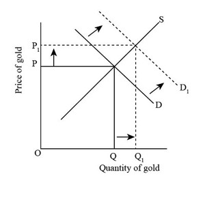
But if suddenly more people immigrate to a certain territory, then the whole curve will shift up and to the right (that is, rise), because new demand will be created – interest in the given product will increase . The same is true with a reversed sign.
Graph 3: Shift of the Demand Curve
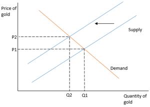
In the complex world of gold trading, multiple prices exist, each influenced by changes in supply. For instance, last year’s refinery shutdowns led to a significant price surge. This increase was a direct result of the work stoppage, which caused the entire supply curve to shift to the left due to a decrease in overall supply.
Conversely, let’s consider a scenario where, instead of refineries closing, new gold mines were discovered and production ramped up. In this case, the supply curve would move to the right, indicating an increase in supply. This example should give you a clearer understanding of how the supply curve responds to changes in production, showcasing its dynamic nature in relation to shifts in market supply.
Graph 4 : Movement of the supply curve to the right
Price Elasticity of Demand and Supply
Supply and demand curves each possess a distinctive slope, which is influenced by their respective elasticities. This means there are two key concepts to consider: the elasticity of supply and the elasticity of demand. These elasticities determine how steep or flat the supply and demand curves are, reflecting the sensitivity of quantity supplied and demanded to changes in price.
Elasticity of Demand
Demand elasticity illustrates how changes in price influence the quantity of a product demanded. Taking our hypothetical gold market as an example, if the price elasticity is -2, this indicates that a 1% increase in the price of gold results in a 2% decrease in its demand.
This percentage change in quantity demanded is a direct observation of demand elasticity
Elasticity is mirrored in the slope of the demand curve. A horizontal demand curve signifies perfectly elastic demand, where at a certain price point, say $1,400 for gold, demand becomes infinite.
This phenomenon is evident through the behavior of the curve. Conversely, perfectly inelastic demand occurs when quantity demanded remains unchanged regardless of price fluctuations, represented by a vertical demand curve.
Typically, demand elasticity reveals how easily consumers can substitute one product for another. Economics textbooks frequently cite the interchangeability of coffee and tea as examples of products with elastic demand. Should the price of one increase, consumers might switch to the other due to their similar benefits. In contrast, addictive products, such as fuels, exhibit inelastic demand, making them prime targets for excise taxes due to their relatively unchanging consumption patterns despite price changes.
Elasticity of Supply
Similar to demand, the elasticity of supply quantifies how a change in price impacts the quantity of goods produced. This concept encompasses scenarios of perfect elasticity (where an unlimited quantity of a good can be supplied at a specific price) and perfect inelasticity (where the quantity supplied remains unchanged regardless of price variations).
Products deemed to have a price elasticity greater than 1 are categorized as relatively elastic. These are goods that can be easily produced, allowing their supply to adjust swiftly in response to price changes. For such products, the quantity supplied changes at a rate greater than that of the price change.
Conversely, products with an elasticity of less than 1 are considered relatively inelastic. In this case, the supply of these goods is less responsive to price changes, exhibiting the opposite behaviour compared to relatively elastic products.
The Paradox of Value: What Does the Law of Supply and Demand Not Explain?
The law of supply and demand, a cornerstone concept introduced by proponents of the classical school of economics, aims to elucidate the rationale behind price formations. This law excellently accounts for the dynamics of pricing, yet it falls short of explaining certain economic phenomena.
One notable example is the variation in prices between different types of goods, particularly the disparity between necessities and luxury items. A classic illustration of this is the comparison between water and gold. While water is fundamentally essential for survival, its market value is significantly lower than that of gold, a luxury item.
This discrepancy is referred to in economics as the “paradox of value.” Both classical and neoclassical economists have struggled to adequately address this paradox, facing considerable theoretical challenges as a result. The underlying reasons for this phenomenon are further explored in discussions about value.
Conclusion
The essence of the law of supply and demand lies in understanding the intricate relationship between prices and the quantity of goods demanded. It highlights how production constraints or policy changes can directly influence price movements, providing a clear framework for explaining these shifts.
This principle encompasses two fundamental laws that illuminate a wide array of effects, both in theory and practical scenarios.
Numerous examples underscore its relevance, such as the impact of refinery and mine operations on gold prices, or how fluctuations in harvests and chip shortages in the market are anticipated outcomes.
The law of supply and demand is a foundational pillar of economics, offering deep insights into why prices fluctuate and how economic activities are interlinked. Through exploring the dynamics of the demand curve and the supply curve, we gain a comprehensive understanding of their pivotal roles in shaping economic processes.
Gold price (XAU-GBP)
3,032.15 GBP/oz
- GBP55.55
Silver price (XAG-GBP)
43.21 GBP/oz
- GBP2.00